Interactive Refraction Statics
New Interactive Refraction Statics module is an interactive environment to complete the workflow of evaluation of refraction static corrections in a fully controllable way — from first break picking, through refraction branch assignment, velocity modeling and, finally, calculation of the statics.
A standard RadExPro Professional license includes 100 launches of the module. You can use this launches both for evaluation/educational purposes and for commercial projects. After the 100 launches are over, this module will require a separate license.
The workflow is divided by several Stages, the Wizard-like module interface will guide you through them:
Stage 0 — The Preparatory One
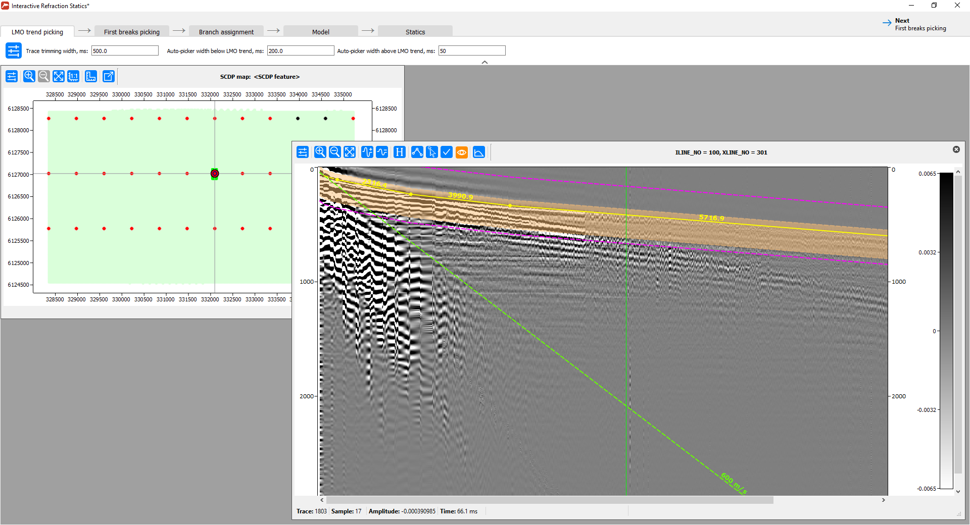
General LMO Trend Picking
On the next stage, you will be working with a small section of the traces around the first breaks, trimmed along the trend. Magenta lines on the figure indicate the edges of the section to be trimmed, while orange-colored area shows the window for automatic search for first breaks. You can independently adjust the width of this window above and below the LMO trend.
Stage 1
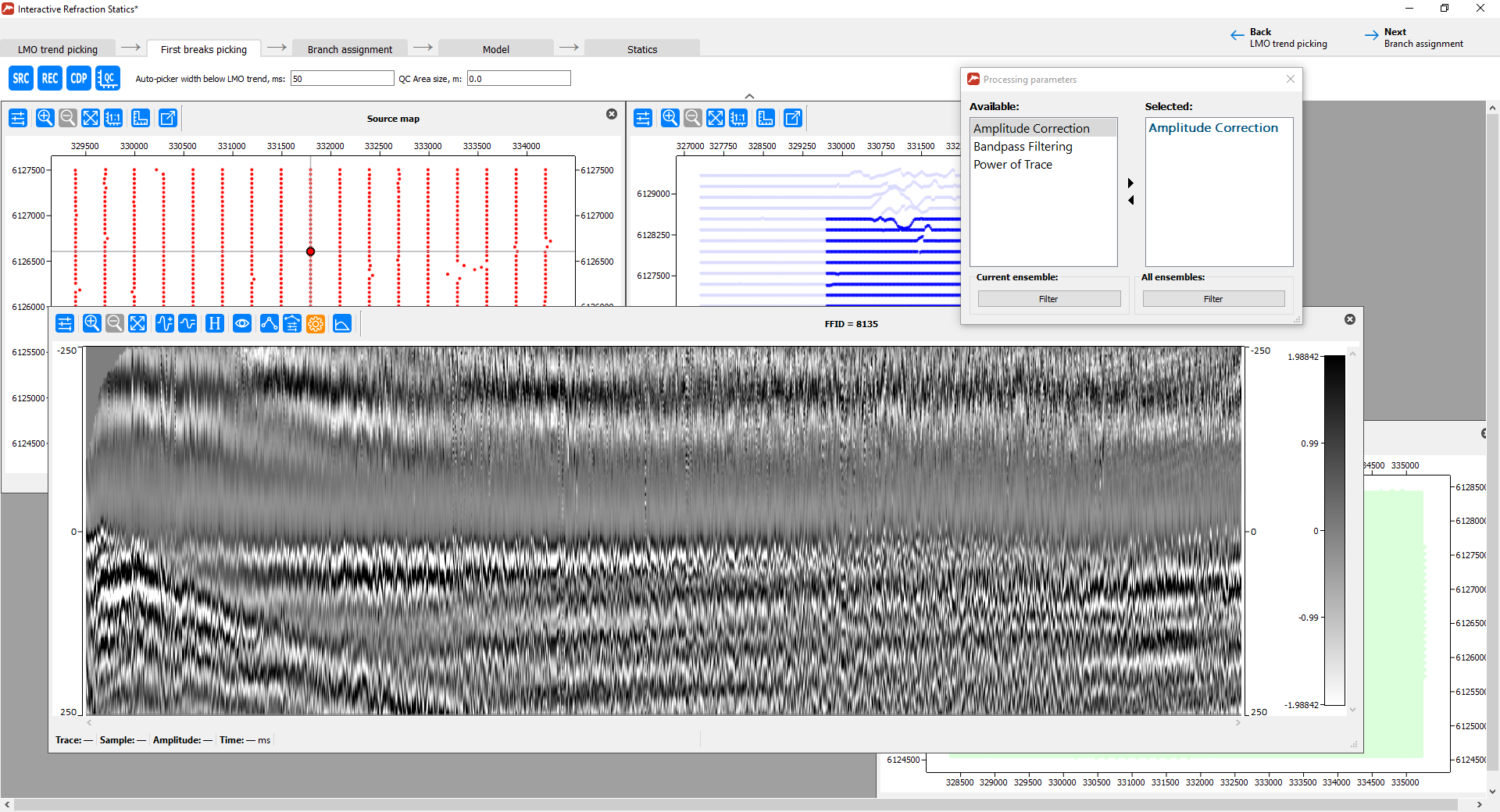
First Break Picking
You will be working with a small section of the traces around the first breaks with LMO-correction applied. You can make some simple pre-processing of the trimmed segment of the data to balance the amplitudes and improve signal-to-noise level:
When the data is ready, you can start picking first breaks using one of the several auto-picking algorithms implemented:
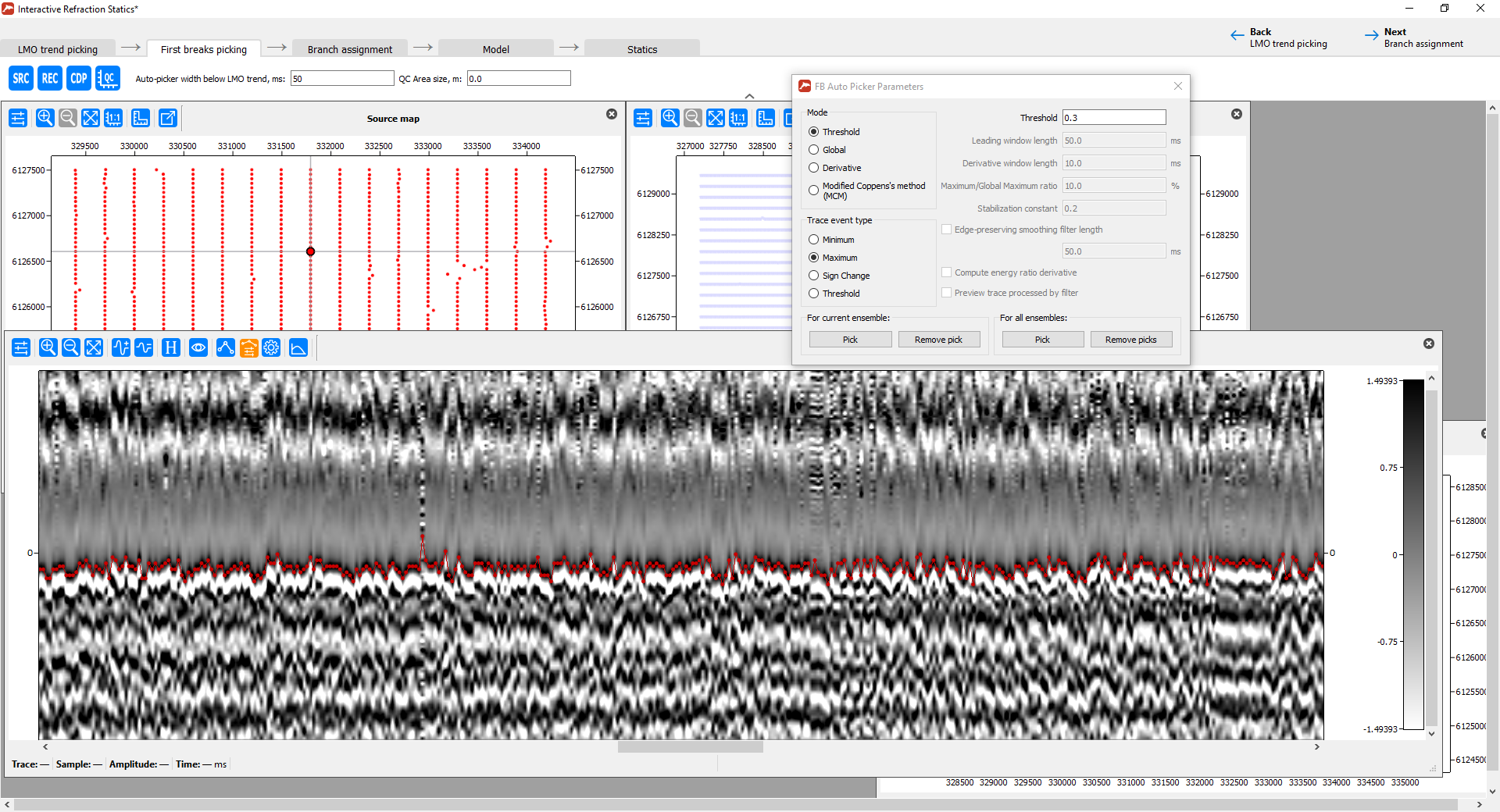
The resulting pick can also be edited manually.
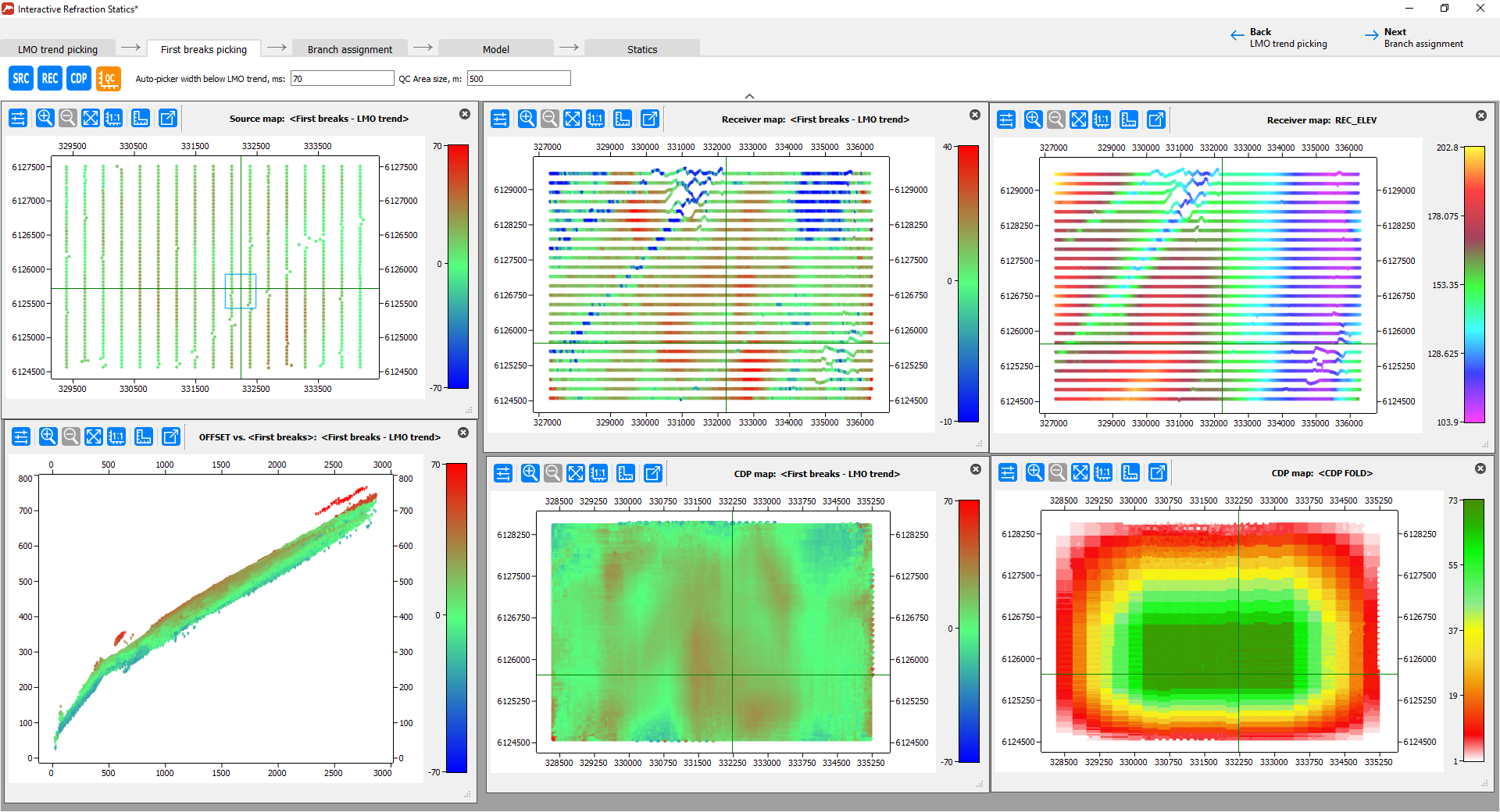
You will enjoy user-friendly and efficient tools to QC the resulting first break pick: you can display first breaks on TWT vs. offset crossplots for super-seismograms in either common shot, common receiver or CDP domains. In case of suspicious picks, you can call the corresponding seismogram directly from the crossplot and edit the picks when needed. Various attribute maps can also help.
Stage 2
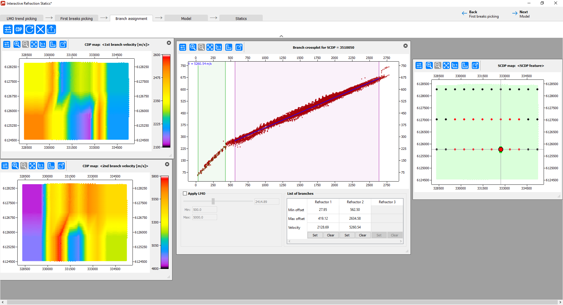
Refractor Branches Assignment
You will be working with the first breaks of super-CDP gathers on TWT vs. offset crossplots indicating branches for each refractor. You can QC the process through maps of velocities, minimum/maximum offsets for each refractor and other attributes. The maps are updated automatically.
When going to the next stage, a velocity model will be calculated.
Stage 3
Velocity Model Display
You can examine resulting velocities and depths/elevations of all refractors. Here you can smooth the first refractor surface before moving next to evaluation of static corrections.
Stage 4
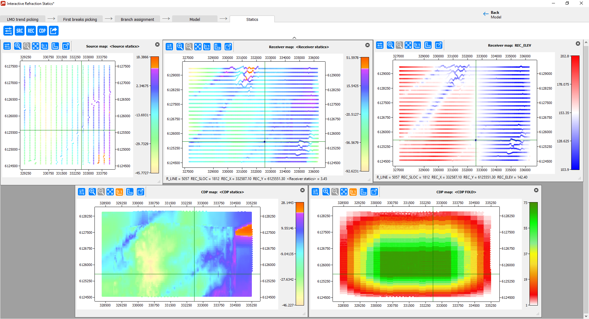
The Result Is Ready!
You can examine resulting static corrections on maps, compare them with topography and other attributes.
Here you can also preview how the statics will affect the data when applied to either common shot, common receiver or CDP gathers, to assess the quality of the result.
Here is the original common-shot gather (as sorted by offset):
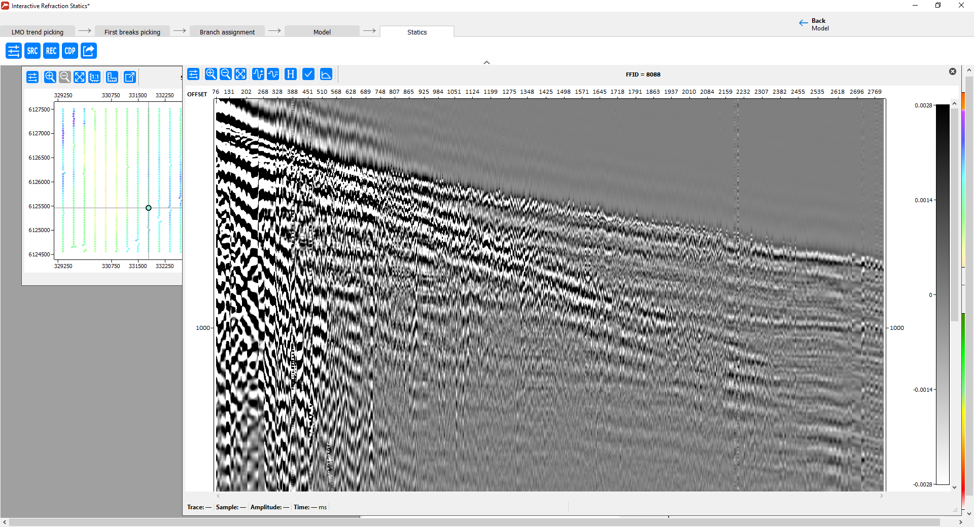
Here is the same gather with the statics applied:
